Mahalanobis Cosine Similarity

This blog post was produced by reading a paper and asking questions to Opus 4.6, and reviewing my Linear Algebra notes.

Some researchers at Columbia and Stanford just released a great paper called The Truthfulness Spectrum Hypothesis. I won't cover the main findings here, but instead focus on one of the techniques they use: Mahalanobis cosine similarity.

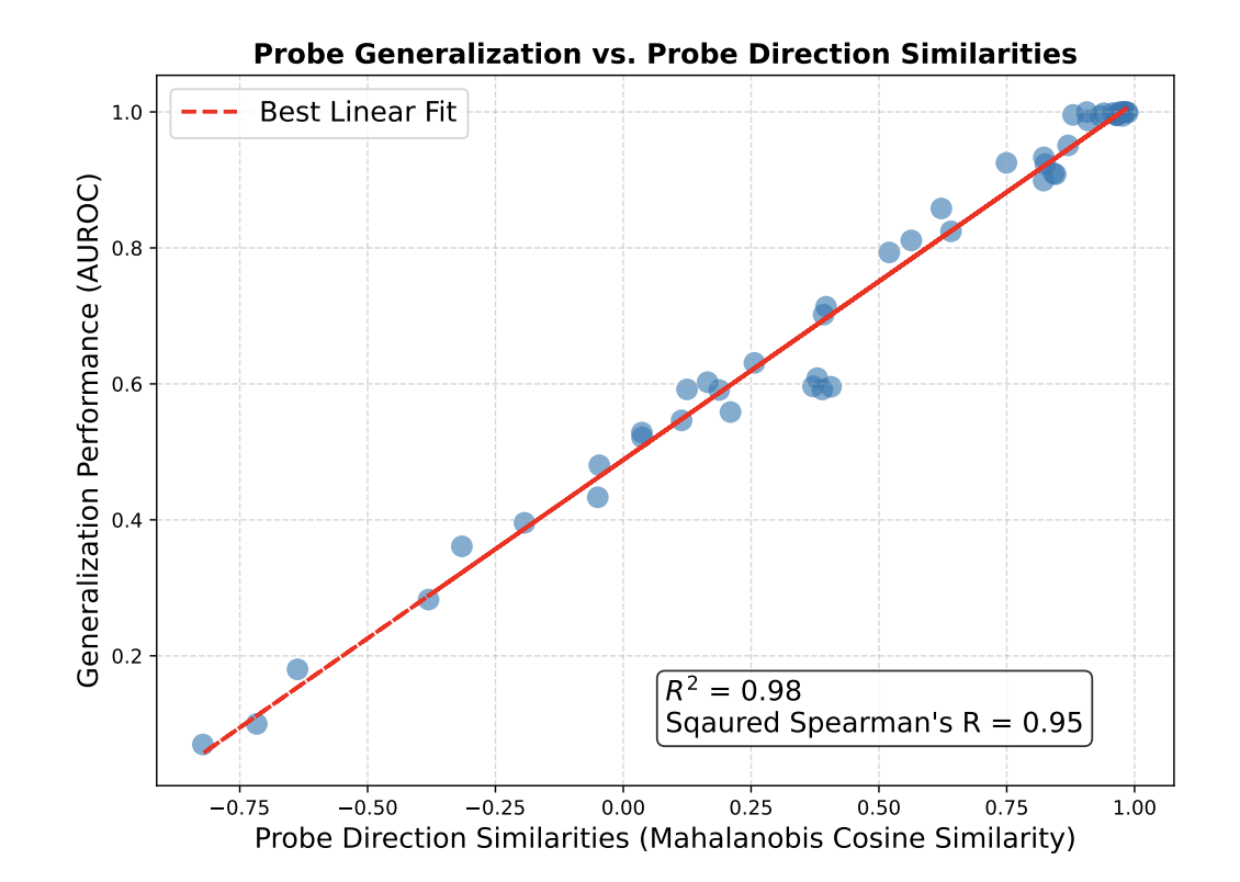
For two probes on different domains, Mahalanobis cosine similarity does a much better job than naive cosine similarity at predicting generalization performance from one probe's performance to the other's:

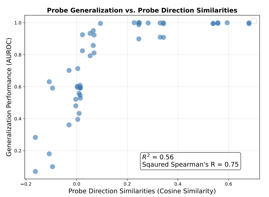
Mahalanobis cosine similarity is an almost perfect linear predictor of cross-domain AUROC ($R^2$ = 0.98, squared Spearman $\rho^2$=0.95), far exceeding standard cosine similarity ($R^2$=0.56, $\rho^2$=0.75; Figure 18, Appendix D).

In other words, the cosine similarity between probes on two different domains performs relatively poorly, while the Mahalanobis cosine similarity does great. Compare the graphs:

What is Mahalanobis cosine similarity?

A limited dataset will not vary across all of the dimensions of the embedding space. Thus, cosine similarity between probe directions takes into account a ton of dimensions that don't actually matter for discriminating on your dataset; by varying those dimensions, you could get two probes with extremely low cosine similarity that both essentially capture the same information on the test set. (e.g. see the standard cosine similarity plot: there's a probe pair with cosine similarity ~0.15 but generalization performance ~100%).

To solve this, Mahalanobis cosine similarity reweights cosine similarity so that it only focuses on the effective dimensionality of the dataset: directions of high variance in the dataset get scaled up, while directions of low variance get compressed. To do this, all you need to do is multiply your input vectors (here $v, w \in \mathbb{R}^n$) by the the covariance matrix of activations on the test set, and normalize appropriately: $$Cos_\Sigma(v, w) = \frac{v^\top \sum_\text{test}w}{\sqrt{v^\top\Sigma_\text{test}v}\sqrt{w^\top \Sigma_\text{test}w}}$$ (For convenience, I'm going to denote $\Sigma_\text{test}=\Sigma$ for the remainder of this post)

Why would this work? To recap some probability theory, in the standard basis, our covariance matrix $\Sigma$ is the $n \times n$ matrix containing the variance of each dimension of $\mathbb{R}^n$ on the test set on the diagonals, and off-diagonal entries being the covariances of each dimension with each other dimension:

$$\Sigma_\text{test} = \begin{bmatrix} \text{Var}(X_1) & \text{Cov}(X_1, X_2) & ... & \text{Cov}(X_1,X_n)\\ \text{Cov}(X_2, X_1) & \text{Var}(X_2) & & \vdots \\ \vdots & & \ddots \\ \text{Cov}(X_n, X_1) & ... & & \text{Var}(X_n) \end{bmatrix}$$

where $X_i$ is the $i$-th dimension of the test dataset, each dimension treated as a random variable. This matrix clearly has something to do with the variance of the dimensions of the data, but it's not obvious that simply multiplying it should 'scale by the dimensions of variance' until we dig a little deeper.

Covariance, Mahalanobis, and the spectral theorem

The important part here is actually one of linear algebra's important results, the spectral theorem:

Spectral Theorem Every real symmetric matrix is diagonalizable (and thus has an Eigendecomposition).

Variances and covariances are real values, and since $\text{Cov}(A,B) = \text{Cov}(B,A)$, our matrix $\Sigma$ is symmetric. Thus, $\Sigma$ is diagonalizable by the spectral theorem. Because it is diagonalizable, we can write an eigendecomposition for $\Sigma$:$$\Sigma = Q\Lambda Q^\top$$ where $Q$ is orthonormal (i.e. a rotation) and $\Lambda$ is a diagonal matrix (i.e. it only scales the basis dimensions). Now, we're still looking at the same dataset -- we've just rotated into a new basis where none of the dimensions have any covariance with one another. $\Lambda$ is the covariance matrix for this new basis: it's the covariance matrix of a new set of variables $\mathbf{Y} = {Y_1, ..., Y_n}$ that we define s.t. each $Y_i$ takes on scalar values representing the $i$th dimension of each point in the dataset. Each $Y_i$ is now uncorrelated with each other $Y_i$ — though not necessarily independent.

What $\Lambda$ does is simple: it finds the directions in this new basis that vary the most on the dataset. Not all of these directions are important for detecting truthfulness; the directions we care about might not be the ones with the largest variance (though it's possible they will be). The important part is just that, when we calculate cosine similarity, now the directions in this subspace with high variance will not get averaged out as much. They get extra weight in our cosine similarity calculations, because we literally just multiplied by their variances, which will be much larger than those of the low-variance directions. (We don't have to worry about the magnitude change, since we divide that out by applying $\Sigma$ in the denominator as well.)

So in sum: in the numerator, when we apply $(v^\top Q) \Lambda (Q^\top w)$, what we're doing is taking $w$ and $v^\top$, rotating them into this new basis by applying $Q^\top$ or $Q$ accordingly, increasing the weight of high-variance directions with $\Lambda$, and then taking the dot product with this scaling.

One last thing is worth exploring: why can't we do this reweighting naively on the original dimensions? Why do we need a diagonal matrix?

Can we just reweight in the standard basis?

Suppose we applied a reweighting matrix $A$ without rotating into the new basis. Let's compare the equations in the dot product: $$v^\top A w = \sum_i v_i \big(\sum_j A_{ij} w_j\big)$$This is a double sum (evil), required because of the matrix multiply we did with $Aw$. In contrast, let's consider the equations in the dot product for our new basis: $$v^\top Q\Lambda Q^\top w = \tilde v ^\top \Lambda \tilde w = \sum_i \tilde v_i \big(\sum_j \Lambda_{ij} \tilde w_j\big) = \sum_i \lambda_i \tilde v_i \tilde w_i$$ because $\lambda_{ij} = 0$ for $i \neq j$.

So we could apply the reweighting in the standard basis -- but it would mess with interpreting cosine similarity, because we wouldn't know which dimensions contribute how much; we don't know which dimensions are actually similar, because every dimension interacts with every other dimension. In contrast, in the rotated $Q$-basis, the cosine similarity behaves nicely: we can just look at our probes in this basis, and see which direction in our latent space is getting picked up by the cosine similarity. This allows us to simply observe those directions, and test whether there are nice linear representations!

Fictional Example

To cement intuition, let's consider a fictional example that's similar to what's going on in the paper. Suppose we have a representation of truthfulness that moves along a manifold embedded in a 10-dimensional subspace of our 8192-dimensional latent space. (This 10-dimensional subspace is not aligned with the basis dimensions.) Some of the remaining 8182 dimensions vary a lot, since the dataset encompasses truthfulness in lots of domains and the semantic content changes a lot, and some of the 8182 dimensions are relatively unchanging for our dataset. We have two probes pointing in exactly the same direction within our 10d subspaces, and suppose they vary ~randomly in the remaining dimensions.

Our normal cosine similarity will capture some of the probe similarity, because they're correlated within that subspace, but the 10 dimensions on which they have high dot product will be annihilated by the remaining 8182 dimensions that are taken into account in the denominator, making their cosine similarity nontrivial, but small. But when we take the cosine similarity in our rescaled version, the high-variance directions are scaled up, and are no longer annihilated; the signal between our probes is detectable by cosine similarity, rather than getting washed out by the denominator's averaging.

Last notes

This doesn't actually explain the linear correlation, just gives an intuition for why Mahalanobis cosine similarity should perform significantly better than standard cosine similarity.

Some bonus thoughts I had while writing this post:

• Thinking through this Mahalanobis question indicated to me the importance of feature geometry; while I was struggling with manifold-rotating in my head, I was really wishing I had some vague intuition about what kind of shape this truthfulness subspace might take on, and whether the intuition I had about e.g. a 4-dimensional manifold embedded in 10-dimensional subspace was plausible or totally contrived. Feature geometry can give you confidence about the kinds of statistics you can use, the kinds of methods that will give you accurate signal about the internals.
• You can interpret $\Sigma$ as a single linear operation — taking $w$ to the eigenspace, applying $\Lambda$, and then moving it back — but that doesn't really help with intuition, because you want to be performing the cosine similarity in the eigenspace for it to make sense. It's easier if you think about it as moving $v^\top$ into the eigenspace with $Q$ and $w$ into the eigenspace with $Q^\top$. But the question then arises: why does $Q$ take $v^\top$ into the same eigenspace? You can answer this by just taking the transpose — since you want to take the dot product by transposing the vector on the left, write $Q^\top v$ as you wrote $Q^\top w$ and then transpose to get $v^\top Q$ — but this is an algebraic operation that doesn't really tell you much, and hides the actual stuff going on. Another way to think about this is that $v^\top$ is a linear functional, since applying it to $w$ gives you a scalar. The Riesz representation theorem gives you an isomorphism between $\mathbb{R}^n$ and its dual space $(\mathbb{R}^n)^*$, and the transpose of $v$ is just its covector under the standard inner product ($v^\top$ is notation for the linear functional $\langle v, - \rangle$). Then $Q$ is the adjoint map or dual map of $Q^\top$, operating in the dual space. This is what the transpose actually means. There's more to talk about here, but not now.