Do Sparse Autoencoders Capture Line Breaking?
Replicating and extending Do Sparse Autoencoders Capture Concept Manfolds? by Bhalla et al.
This blog post is a work in progress replication and extension of Do Sparse Autoencoders Capture Concept Manfolds? by Bhalla et al. It's a total mess, because I'm still working on the project and am really excited about running experiments, less so about actually paper-writing. You can see and use the codebase here.
Model representations are not, in fact, linear; representations of many concepts lie on manifolds, not simply in linear directions; linearity is an occasional byproduct when a manifold has nice linear separability-ish properties.
Bhalla et al. at Goodfire recently released a paper that asks the question, how well do sparse autoencoder features capture nonlinear geometry? Obviously SAE features are linear — the question is, how do these linear features relate to underlying semantic manifolds. The paper describes three regimes that look approximately as follows:
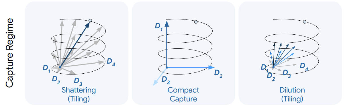
It tests the conditions under which SAEs fall into these distinct regimes, and finds that the answer depends at least on the size of the number of active features $k$: shattering happens at low $k$, capture has intermediate $k$, and dilution has high $k$. To determine the regime, the paper fits an ising model to SAE co-firing patterns in order to find SAE features that seem to be representing the same manifolds.
I'm super excited about this paper: it's a first step in finding a general method to bootstrap from linear methods to nonlinear geometry. I wanted to see if the method was robust enough to recover the results from Anthropic's When Models Manipulate Manifolds, where they find that the model is performing line breaking by comparing helical line-length manifolds.
Outline for this post:
Step 1. Replicate the full synthetic experiment setup to validate the Ising model implementation, etc.
Step 2. Replicate the major results in a new model context (Gemma 12B) using Gemma Scope 2's suite of well-trained SAEs
Step 3. Validate that Gemma can actually perform the line breaking task (it may be too small or too different to have learned the solution that Haiku has in the Anthropic paper), and then see if we can use the Ising model to determine the family of SAE features, which would give us the subspace in which the line-length helices are located.
Step 1. Synthetic Data
Suppose that the model internals are properly modeled as a mixture of manifold samples — manifold superposition, rather than just linear direction superposition.
Each sample $x$ that we take from our "model internals" will be described by $$x = \sum_{i \in S} \tilde \gamma_i(\theta_i) V_i + \epsilon$$for $S$ an active set of manifolds ($|S|$ be is hyperparameter describing the number of manifolds to include in each sample), $\tilde \gamma_i(\theta_i)$ a point sampled from a normalized manifold, and $V_i$ is an embedding matrix up into $\mathbb{R}^d$ from the manifold itself. ($V_i$ is generated from a decomposition of a random matrix.)
The paper uses 8 types of manifolds (circles, spheres, tori, Mobius strips, Swiss rolls, helices, flat disks, line segments) each with 6 different parameter setups.
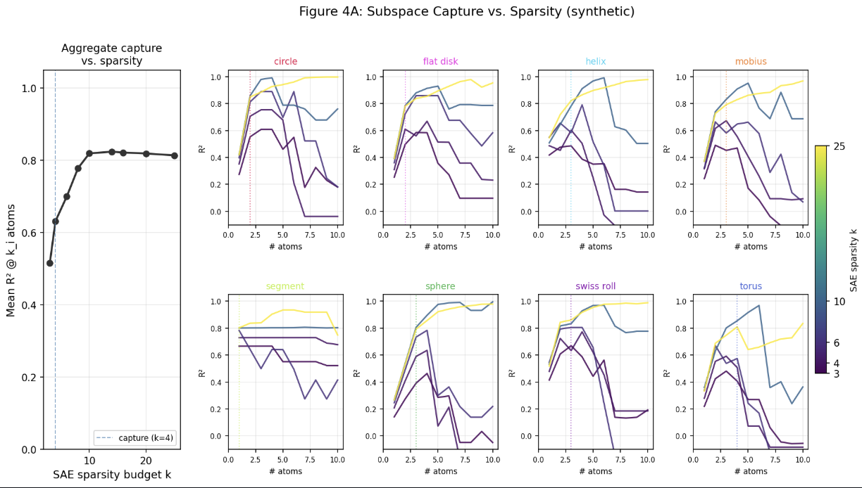
Then for $|S| = 4$ the paper trains sparse autoencoders with overcomplete size $c = 512$, sweeping over $TopK$ sizes $3,4,6,8,10,14,16,20,25$ to show that those different sizes change the regimes.
We end up with this plot:
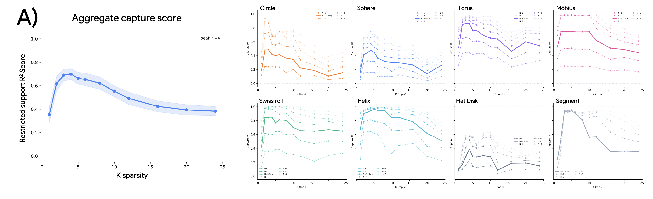
For reference, the corresponding diagram in the original paper is less nice, but broadly quite similar:
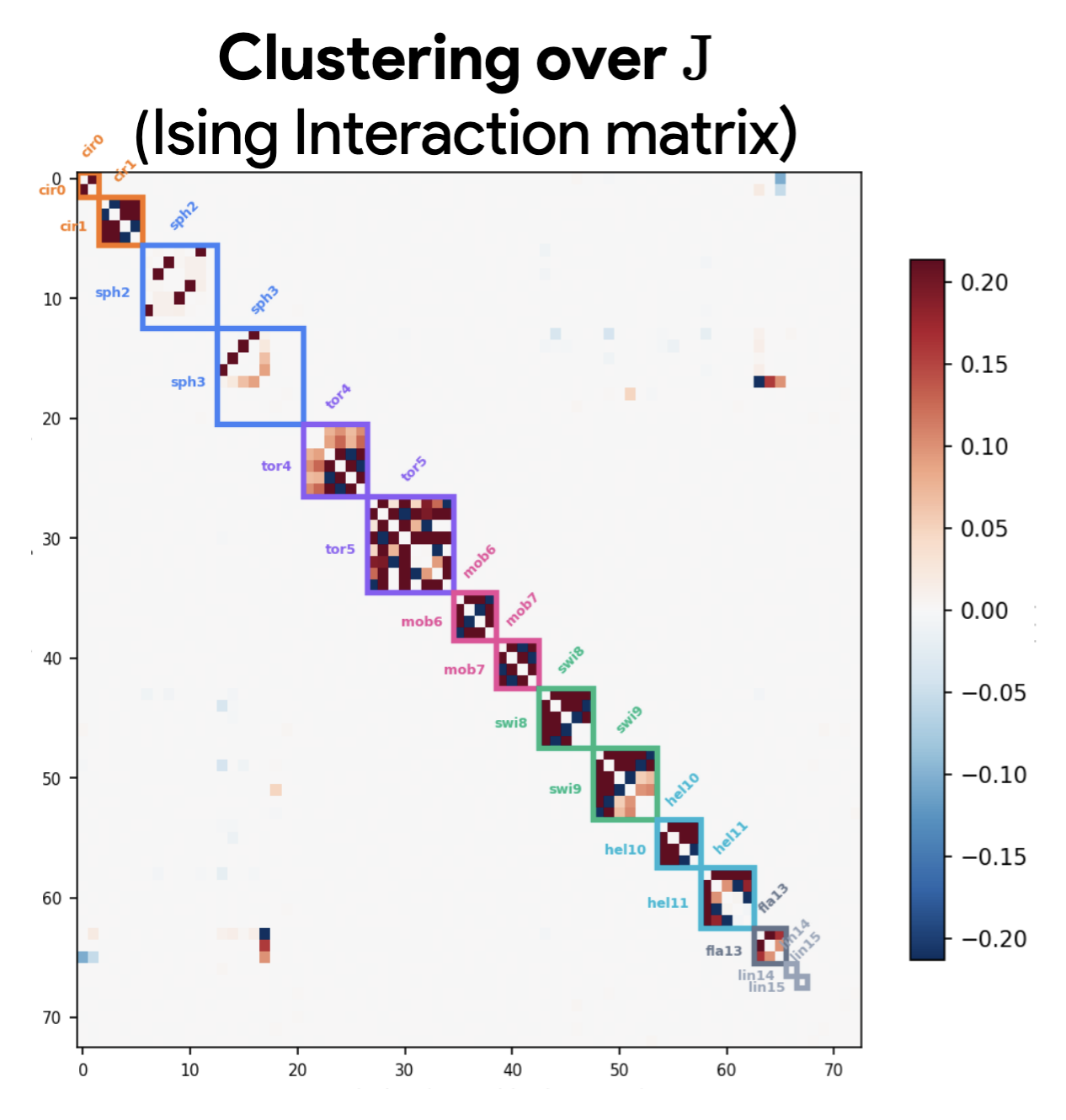
The Ising coupling matrices look quite good as well:
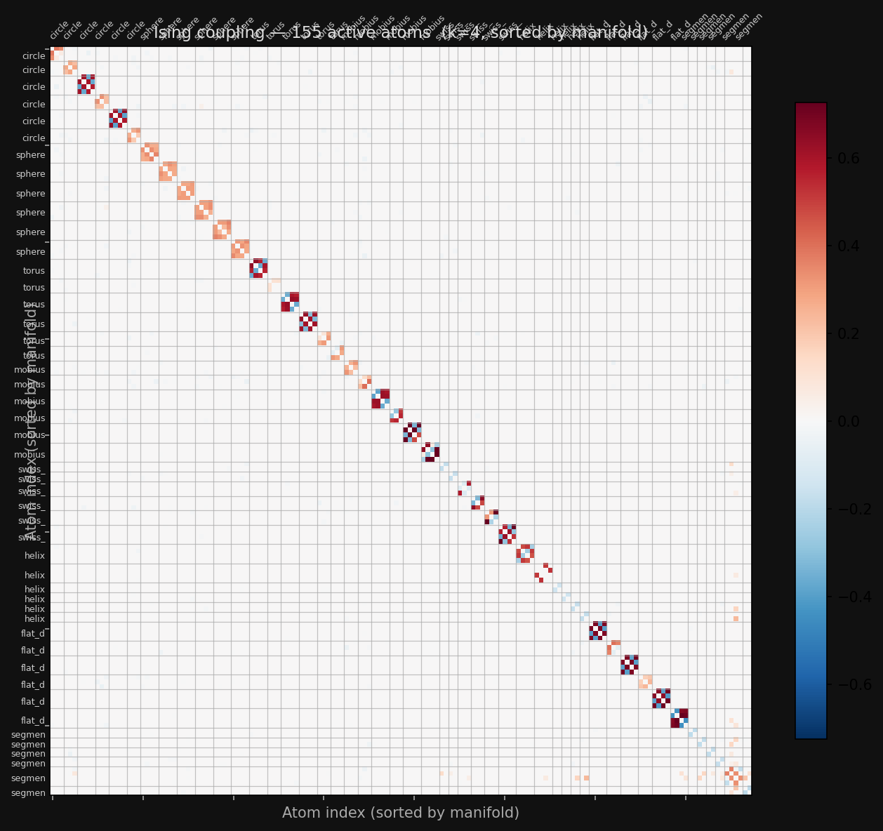
Compared with the original:
Step 2: Replication on Gemma
The original paper trains SAEs from-scratch on Llama 3.1 8B. I didn't want to depend on my skill at training SAEs for this replication, so I decided to replicate on a different model (Gemma 3 12B) which has pretrained high-quality SAEs.
First, we check whether the model actually has the nice manifolds to be discovered?
 |
 |
|---|---|
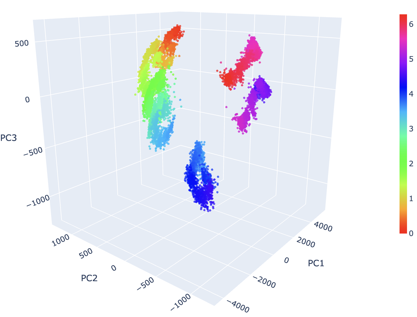
| Above: Colors manifold is not looking nice... (see next section) | Above: Days of the week are ~discrete-circular |
 |
 |
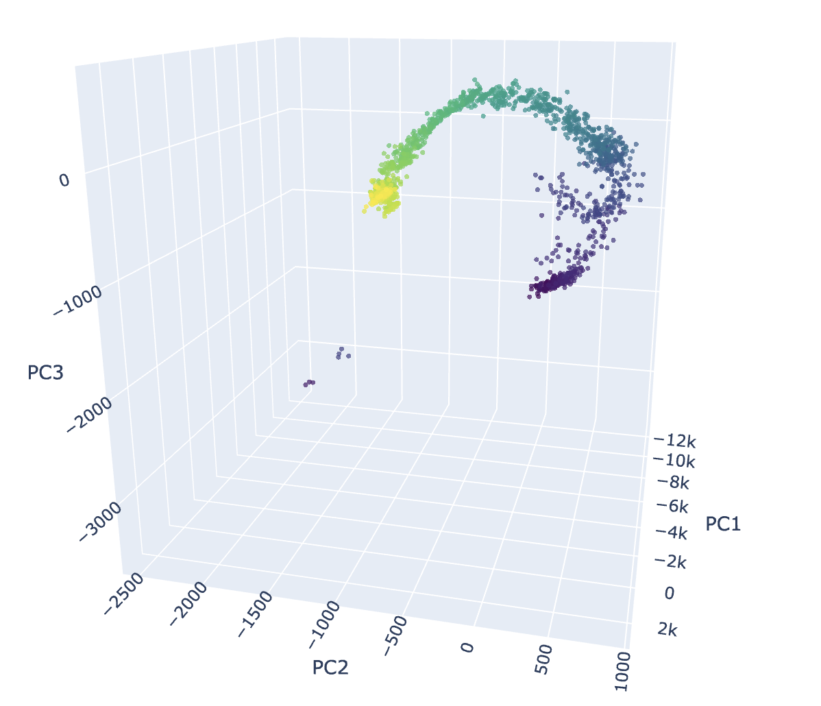
| Above: Temperature (Nicely helical) | Above: Years (Helical) (Actually, I added month+year which gives it extra structure) |
Temperature is clearly quite nice, and years is OK; days of the week is weird and discrete-ish, but shows signs of the circular representation previously described. The colors 'manifold' is grouped into 4 semi-meaningful clusters; the cluster in the corner has low saturation, one of the central clusters has a high saturation, and one of the central clusters has a lot of dark/black colors.
2.1 What's going on with the color manifolds?
I became quite curious about the structure of the color manifold — what's going on with those clusters?
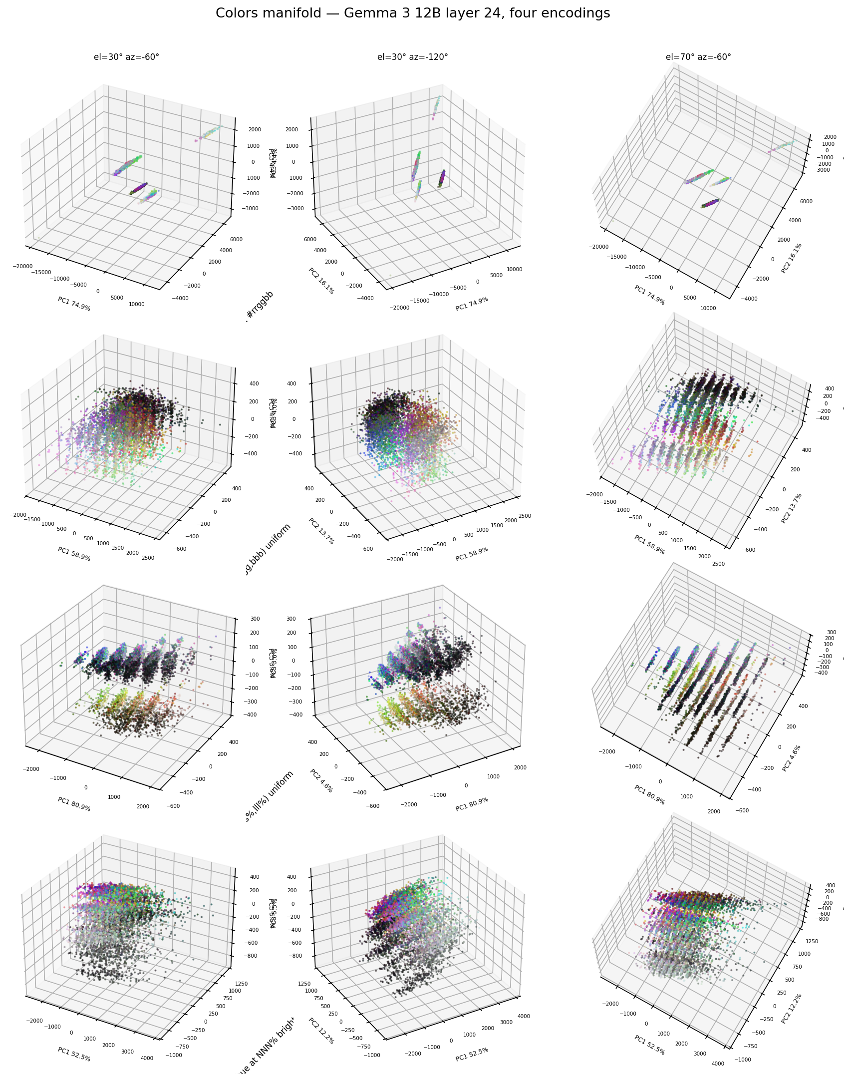
I ran k-means and had Claude inspect the embeddings. It turns out that the clusters are perfectly grouped by embedded length: hex values #rrggbb get split into 4,5,6 and 7 tokens — those sizes provided the 4 manifolds we saw. It's a byte-pair encoding tokenization artifact that substantially alters the representations, even though we're sampling last token of the prompt The hex code #rrggbb is for the color! I was surprised how much the specific format of the colors mattered for the structure of the manifold (see next graph), but this is a very memorization heavy task so maybe that makes sense?
Trying different encodings reveal a wide variety of different structures:
and the structures vary across layers:
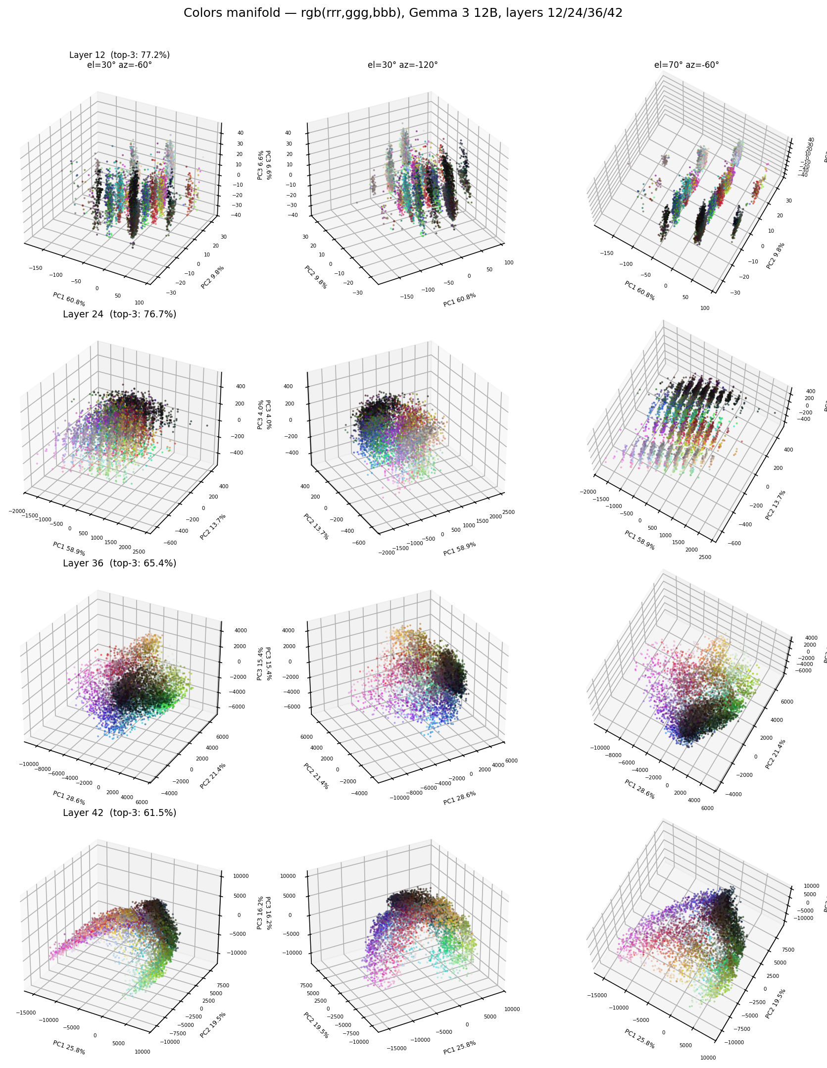
I want to explore the color representations more, this is really interesting. There's a visible process of unpacking and structuring the representations, and I want to understand how that happens.
Can the ising model rediscover our manifolds?
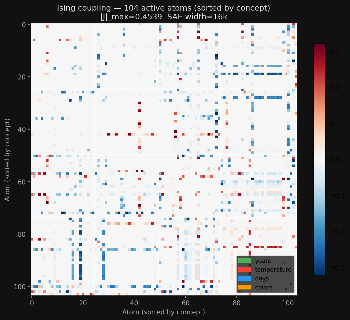
I haven't gotten the ising model working right yet. It currently looks like this:
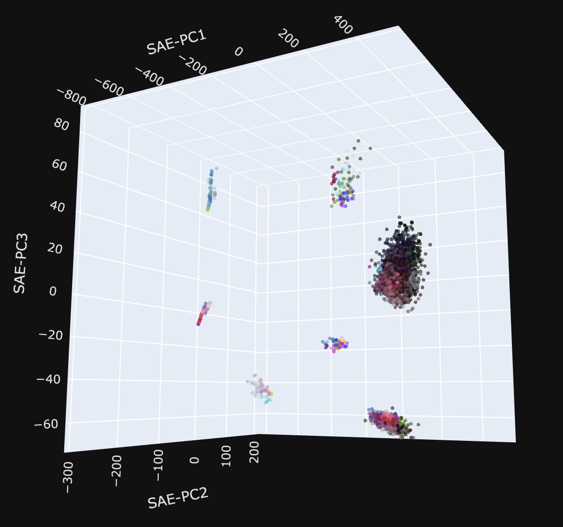
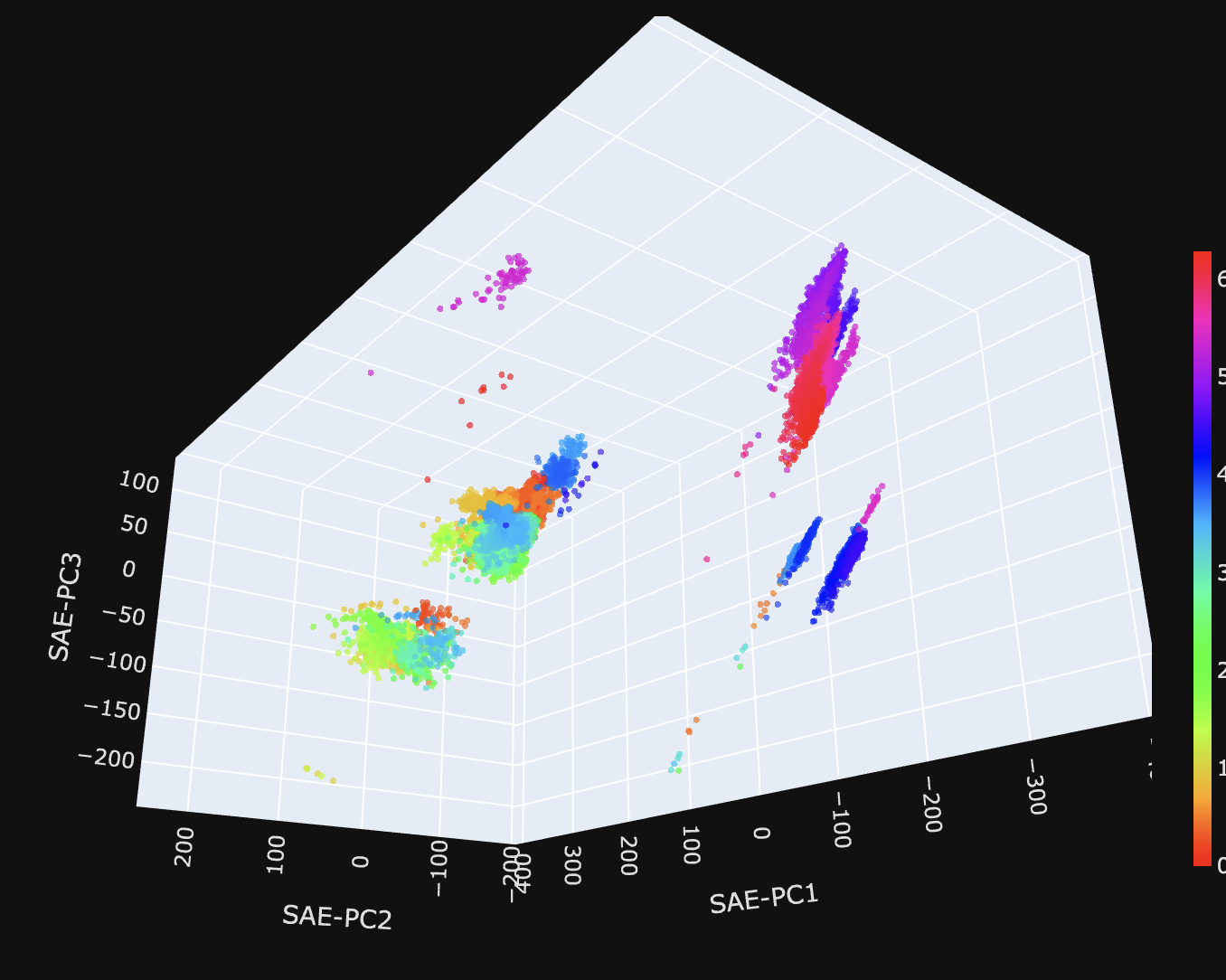
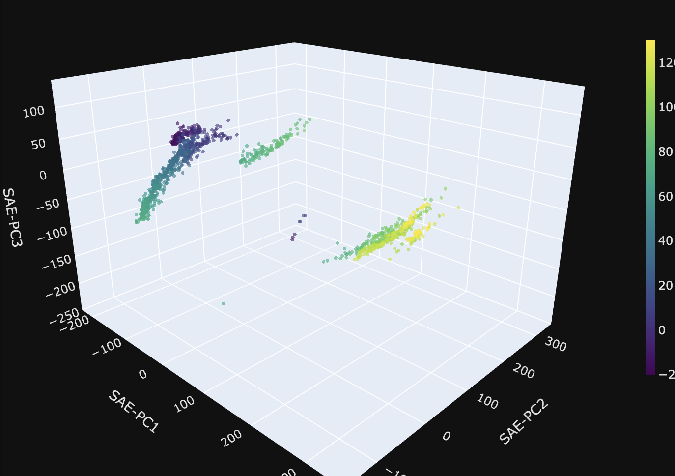
But the SAE does do a good job of capturing our concept manifolds! Here are the plots from before, projected into the space defined by the top 3 SAE features:
 |
 |
|---|---|
| Colors is cooked because the clusters are cooked (need to rerun with non-hex representations) | Days of the week looks... okay? |
 |
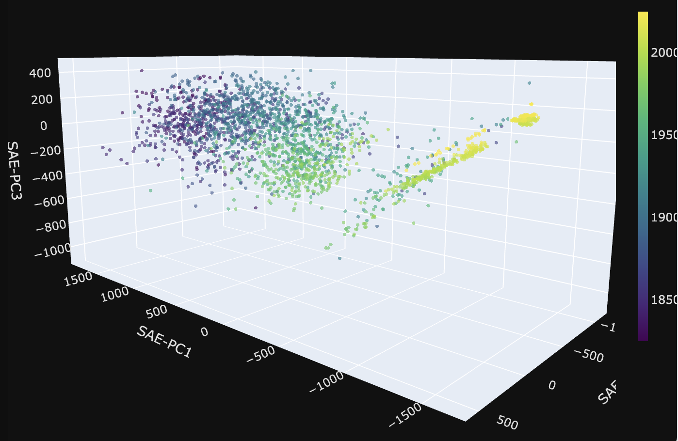 |
| Temperature mostly recovers its curvature, though split into 3 chunks, roughly [-20, 80], [80, 100] and [100, 120] | Years turns out to be beautiful and nearly linear! |
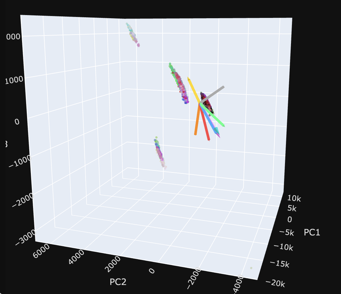
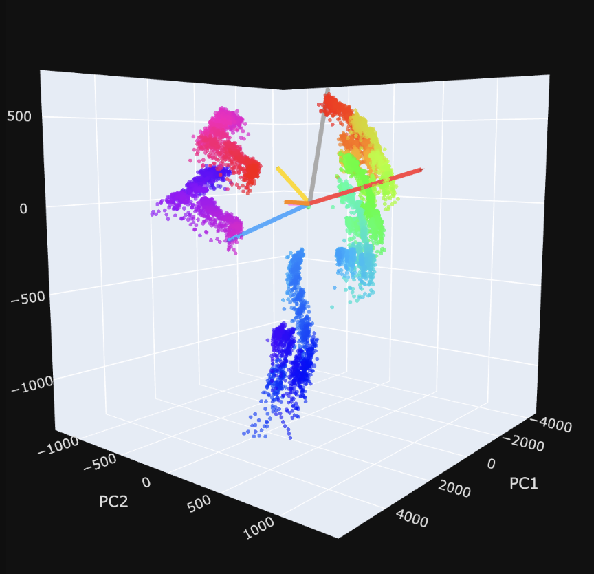
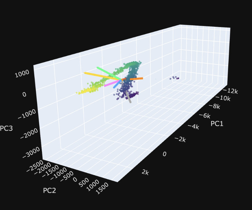
| We can also look at the manifolds again in PCA space, and show our SAE directions in that space: |
 |
 |
|---|---|
 |
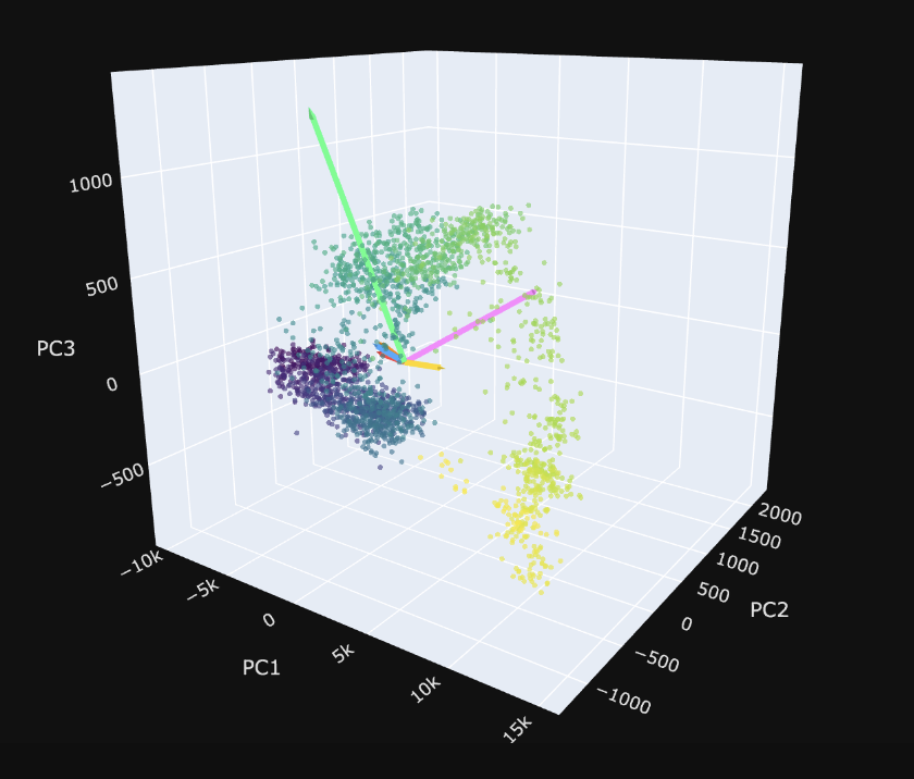 |
The visualization is more informative because you can scroll and you can see the $R^2$ values for the axes.. But my idea here is basically visualizing the shattering/capture/dilution regimes. I need to do a better job weighting the visualization by the 'significance' of the feature, but I like this as a view going forward.
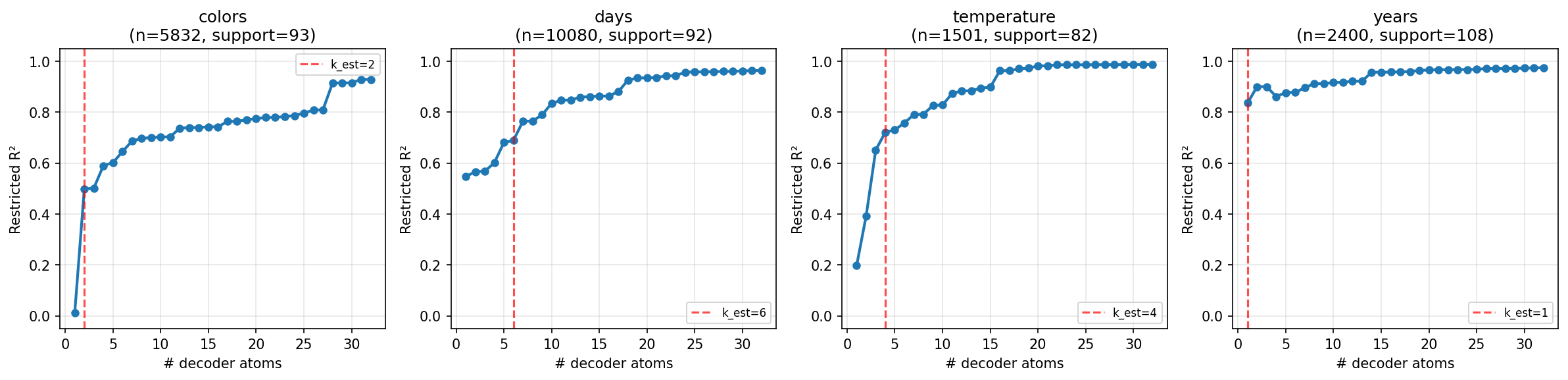
And the restricted $R^2$ gets good after a couple of these features:
Step 3: Line breaking Experiments
I wanted to see if I could recover the results from Anthropic's When Models Manipulate Manifolds using these techniques. This is still in progress — things are looking good so far but I haven't gotten the Ising model right yet.
But there are some promising preliminaries:
3.1 Does Gemma succeed at line breaking?
Yes — not perfectly, but it's quite good. Gemma 27B is better at it, as expected. here's a logit probe looking at log_p(newline) − log_p(word) as we move along the number-of-characters axis:
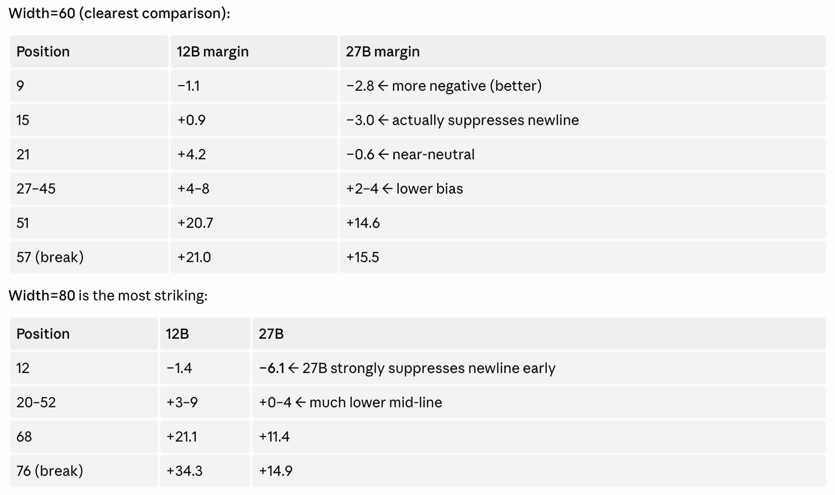
(thanks claude for the nice table).
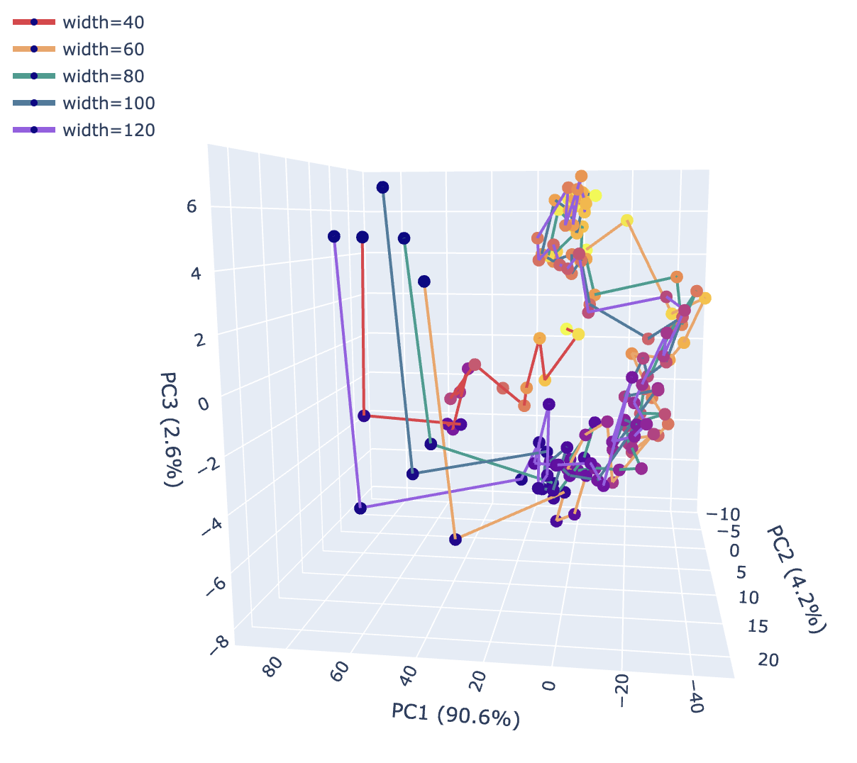
This means that Gemma 12B is more trigger-happy. It tends to break at around 60% of the line's length; Gemma 27B breaks later, around 80%ish. They both occasionally overflow the limit, but overall they're not terrible at the task, and there's strong evidence just from this logit probe that they're actually representing the character position. Here are trajectories through PCA-space in the attention_out in Layer 1 (which as we'll see below is doing a ton of work) for different widths as we move along character position: they look pretty similar!
3.2 Early layer early results
Ok, so how is this happening mechanistically? We can linearly probe for character position with 85% R^2 after the first layer, and 99% after the second layer — seems like we have our answer! This supports the hypothesis that Gemma has a similar mechanism to Haiku in the early layers.
 Probes trained on various components in L0 (first layer) and L1
3.3 Ising matrices
Ok, then can we discover these manifolds autonomously?
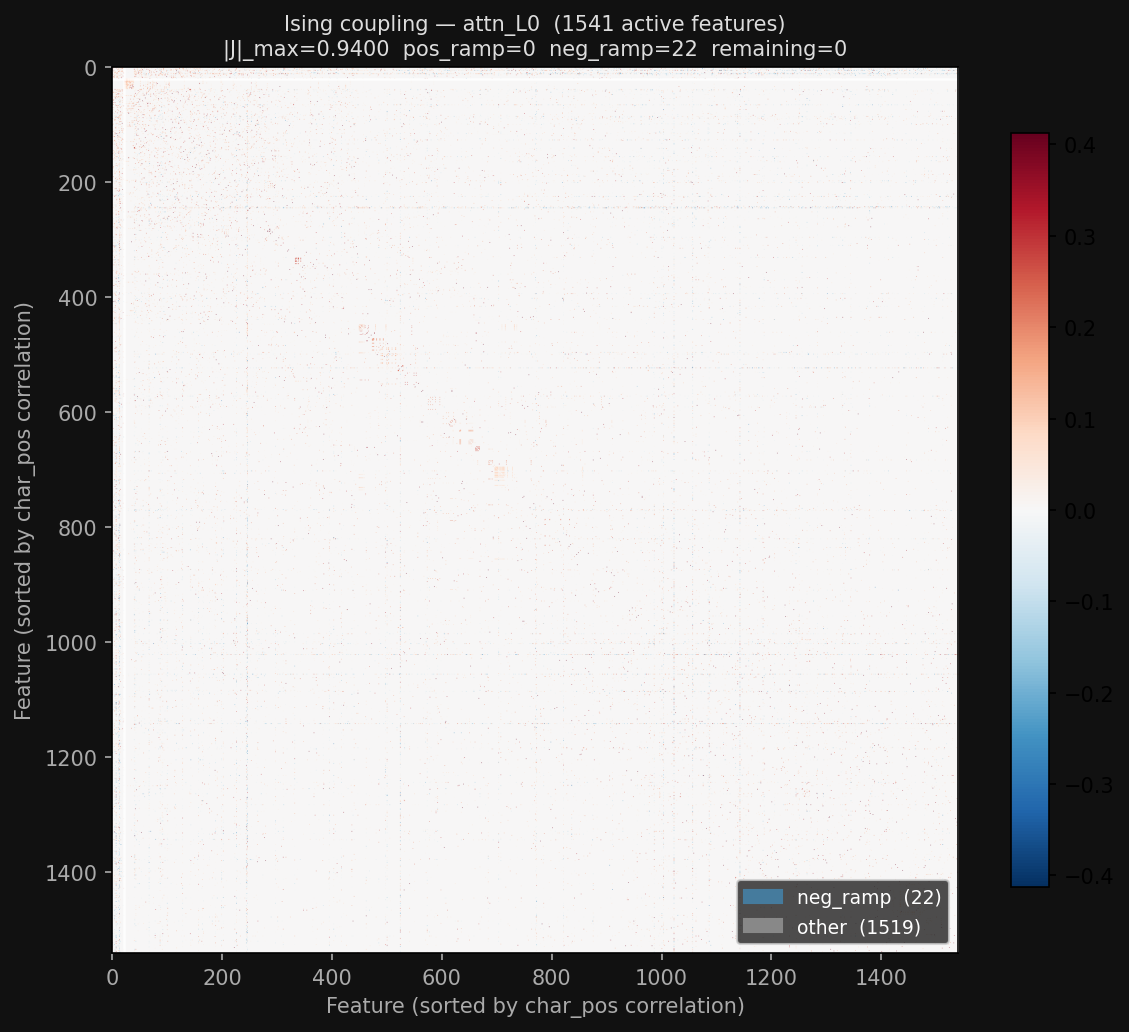
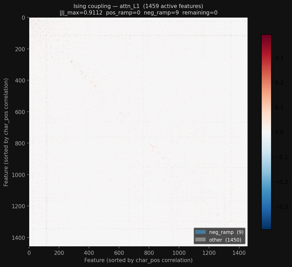
The ising couplings for L0 and L1 attention output SAEs (from Gemma Scope— yes, Gemma Scope has SAEs for ~every component of ~every layer of each of its models, of multiple widths!) are fascinating — if you look closely, there are a couple very nice block structures in the middle of the matrix. (ignore all the extra information on the graphs like neg_ramp, that was me testing a hypothesis I'm not going to describe for now)
But the ising couplings for some other layer (layer 24) in general look pretty bad:
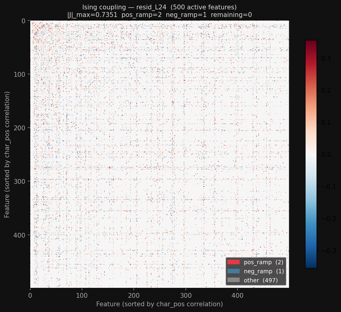
I'm not sure what I'm doing wrong with these couplings. But this suggests an interesting possibility: maybe the couplings do better on layer outputs than the residual stream itself? Could be the case; presumably the layer outputs are less polysemantic than the residual stream in general. But in order to do this analysis I need to have a better understanding of exactly how the ising model works/what properties it has relative to other covariation metrics to say confidently.